Circle bundles and the Hopf fibration

The monopole connection in Connections, flux, and holonomy needed two potentials on a two-sphere. What if we attach the missing phase angle as an actual circular direction? For unit flux, the resulting three-dimensional space is a three-sphere, with a round metric that we can reconstruct explicitly.

Use the geometry of the round three-sphere for its ambient coordinates and global frame. This lesson is geometry on a positive-definite three-manifold. It assumes no Killing spinor or supersymmetric background fields. A circle direction or a bundle number by itself does not count preserved supercharges. The same geometry can also appear as a spatial slice or a factor of a four-dimensional spacetime.

A circle above every point of a sphere

Combine the dimensionless coordinates of the unit three-sphere into two complex numbers:

$$z_1=y^0+iy^1,\qquad z_2=y^2+iy^3, \qquad |z_1|^2+|z_2|^2=1. \tag{T10.1}$$

They are ordinary coordinates, not spinor fields. The physical round metric has radius $\ell>0$ and is $ds^2=\ell^2(|dz_1|^2+|dz_2|^2)$ restricted to the constraint. Define the map

$$\pi(z_1,z_2)=\mathbf n =\left(2\operatorname{Re}(\bar z_1z_2),\, 2\operatorname{Im}(\bar z_1z_2),\, |z_1|^2-|z_2|^2\right). \tag{T10.2}$$

Its image lies on a unit two-sphere because $|\mathbf n|^2=4|z_1|^2|z_2|^2+(|z_1|^2-|z_2|^2)^2=1$. The common phase rotation

$$(z_1,z_2)\longmapsto(e^{i\lambda}z_1,e^{i\lambda}z_2), \qquad \lambda\sim\lambda+2\pi, \tag{T10.3}$$

leaves $\mathbf n$ unchanged. Conversely, $n_3$ fixes both magnitudes and $n_1+in_2$ fixes their relative phase whenever both are nonzero. Only the common phase remains. At a pole one coordinate vanishes, but the nonzero coordinate still has a full phase circle. No point is fixed by a nontrivial common phase.

Thus each inverse image $\pi^{-1}(\mathbf n)$ is one circle. The map is the Hopf fibration, $S^1\to S^3\mathrel{\mathop{\longrightarrow}^{\pi}}S^2$. Here $S^3$ is the total space, $S^2$ the base, and each circle a fiber. A principal circle bundle means that locally the total space looks like a base patch times a circle, with the circle acting freely and transitively on each fiber. We now exhibit those local products and their gluing; a global product is a stronger assertion.

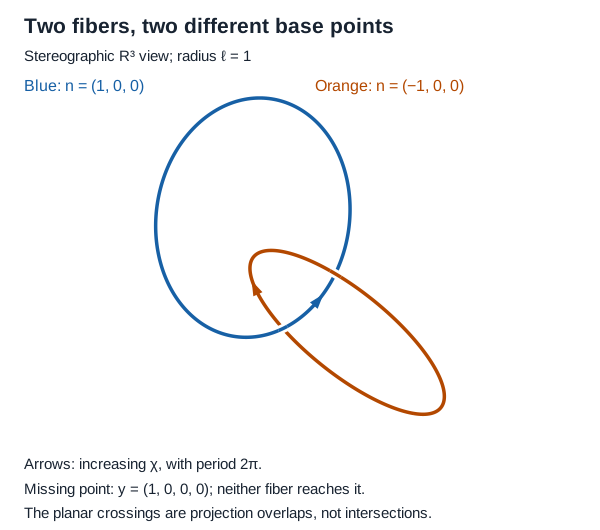
Each whole circle maps to one base point: blue to $(1,0,0)$ and orange to $(-1,0,0)$. The fibers are disjoint in $S^3$; their planar crossings are projection overlaps, not intersections. This stereographic view and its planar drawing do not preserve the sphere’s metric distances: apparent circle sizes are not physical fiber radii. The Hopf-fibration laboratory constructs these fibers and checks the map.

Join the two fiber angles

Write the base coordinates as $\mathbf n=(\sin\theta\cos\varphi,\sin\theta\sin\varphi,\cos\theta)$, with $0\leq\theta\leq\pi$ and $\varphi\sim\varphi+2\pi$. On the patch $U_N$ excluding the south pole choose a representative with $z_1$ positive real:

$$s_N(\theta,\varphi)= \begin{pmatrix}\cos(\theta/2)\\e^{i\varphi}\sin(\theta/2)\end{pmatrix}, \qquad z=e^{i\chi_N}s_N,\qquad\chi_N\sim\chi_N+2\pi. \tag{T10.4}$$

The map $s_N$ is a local section: it selects one point of each fiber. On the southern patch choose instead

$$s_S=\begin{pmatrix}e^{-i\varphi}\cos(\theta/2)\\\sin(\theta/2)\end{pmatrix}, \qquad z=e^{i\chi_S}s_S. \tag{T10.5}$$

These representatives are smooth at their included poles. For example, $s_N=(\sqrt{(1+n_3)/2},\,(n_1+in_2)/\sqrt{2(1+n_3)})^T$ has no singularity near $n_3=1$. On the overlap,

$$s_N=e^{i\varphi}s_S,\qquad \chi_S=\chi_N+\varphi\pmod{2\pi}. \tag{T10.6}$$

The second equation follows by representing the same $z$ in the two products. The circle has not acquired two independent angles. Its coordinate changes when we change which section defines zero phase.

A global connection with local potentials

Define the real one-form on the total space

$$\Theta=-i\left(\bar z_1dz_1+\bar z_2dz_2\right) =y^0dy^1-y^1dy^0+y^2dy^3-y^3dy^2. \tag{T10.7}$$

Reality follows from $d(|z_1|^2+|z_2|^2)=0$. Its polynomial ambient expression is smooth everywhere. It is exactly the earlier global-frame form $\eta^1=e^1/\ell$.

The generator of the common phase is $\xi=(-y^1,y^0,-y^3,y^2)\cdot\partial_y$. Its flow parameter has period $2\pi$, and direct substitution gives $\Theta(\xi)=1$. The form is invariant under the common phase. These two properties make $\Theta$ a normalized principal-circle connection. It specifies which displacements contain a vertical phase change; it is not an additional flavor gauge field or the R-symmetry source of the three-manifold paper.

Substituting the two local representatives gives

$$\begin{aligned} \Theta&=d\chi_N+a_N=d\chi_S+a_S,\\ a_N&=\frac{1-\cos\theta}{2}\,d\varphi, &a_S&=-\frac{1+\cos\theta}{2}\,d\varphi. \end{aligned} \tag{T10.8}$$

For instance, in the north patch the phase derivatives contribute $\cos^2(\theta/2)d\chi_N+\sin^2(\theta/2)(d\chi_N+d\varphi)$; the real amplitude derivatives cancel. Equation (T10.6) then makes the two expressions for $\Theta$ identical. Downstairs the potentials differ by $a_N-a_S=d\varphi$, exactly the unit-flux transition of the connection lesson.

Differentiating removes the fiber coordinate:

$$d\Theta=\pi^*F,\qquad F=da_N=da_S=\frac12\sin\theta\,d\theta\wedge d\varphi. \tag{T10.9}$$

The notation $\pi^*F$ means evaluate the base two-form on the projections of tangent vectors upstairs. It has no component along $\xi$. With the outward base orientation $\sin\theta\,d\theta\wedge d\varphi>0$,

$$\boxed{\displaystyle c_1=\frac1{2\pi}\int_{S^2}F =\frac1{2\pi}\frac12\int_0^\pi\sin\theta\,d\theta \int_0^{2\pi}d\varphi=1.} \tag{T10.10}$$

This is the bundle number in the declared orientation and period normalization. Equivalently, $e^{i\varphi}$ winds once around $U(1)$ on the equator. Reversing the circle action while renormalizing its connection, or reversing the base orientation, reverses this sign.

The connection is global on $S^3$, although no single smooth potential exists on $S^2$. There is no conflict with Stokes’ theorem: the nonzero integral is over the base, where $a_N$ and $a_S$ are only local. In fact, a global section would pull $\Theta$ back to a global base potential with derivative $F$, forcing $\int_{S^2}F=0$. Therefore this bundle has no global section and is not the product bundle $S^2\times S^1$.

The same normalization appears in Closset–Kim, (3.90) and (8.11). We are using an ordinary smooth principal circle bundle. Their more general Seifert examples can have exceptional fibers; those require additional data and are not being assumed here.

Vertical motion and horizontal motion

A vertical vector points along $\xi$ and leaves the base point fixed. A vector $X$ is horizontal if $\Theta(X)=0$. Every tangent vector decomposes uniquely as $X=\Theta(X)\xi+[X-\Theta(X)\xi]$. The second term is horizontal and projects to a base displacement.

In the northern coordinates, horizontal lifts of the coordinate vectors are

$$H_\theta=\partial_\theta,\qquad H_\varphi=\partial_\varphi- \frac{1-\cos\theta}{2}\partial_{\chi_N},\qquad \xi=\partial_{\chi_N}. \tag{T10.11}$$

Going in the base azimuthal direction generally requires compensating motion in the fiber. Their bracket exposes the twist:

$$[H_\theta,H_\varphi] =-\frac12\sin\theta\,\xi, \qquad \Theta([H_\theta,H_\varphi])=-F(\partial_\theta,\partial_\varphi). \tag{T10.12}$$

Two horizontal motions can therefore generate a vertical one. The horizontal planes are transverse to the fibers, but they are not tangent planes to a family of two-dimensional surfaces upstairs. This does not prevent a smooth quotient base. More generally “transverse” need not mean that there is a global transverse slice.

For this example $\Theta\wedge d\Theta$ is nowhere zero; such a one-form is called a contact form. The global frame makes the statement valid even at the angular poles: $\Theta\wedge d\Theta=2\eta^1\wedge\eta^2\wedge\eta^3$. An arbitrary circle-bundle connection need not have this property. No spinor-bilinear construction or transverse complex structure was needed for our calculation.

The round metric follows directly from (T10.4):

$$\begin{aligned} ds^2&=\ell^2\left[\frac14d\theta^2 +\cos^2\frac\theta2\,d\chi_N^2 +\sin^2\frac\theta2\,(d\chi_N+d\varphi)^2\right]\\ &=\ell^2\Theta^2+ \frac{\ell^2}{4}\left(d\theta^2+\sin^2\theta\,d\varphi^2\right). \end{aligned} \tag{T10.13}$$

Thus the fibers have circumference $2\pi\ell$, the unit vertical vector is $\xi/\ell$, and the base with its quotient metric is a round sphere of radius $\ell/2$. The dimensionless unit vector $\mathbf n$ did not set the physical base radius. The connection $\Theta$ is normalized by a group period; the metric-unit one-form is instead $\ell\Theta$.

The volume check keeps both radii: $\operatorname{Vol}(S^3_\ell)=(2\pi\ell)\,4\pi(\ell/2)^2=2\pi^2\ell^3$. This agrees with the independent ambient-coordinate calculation. All of $\theta,\varphi,\chi_N$ are dimensionless angles, while $\ell$ has length units.

The source paper’s metric (5.11) uses an angle $\psi_P$ of period $4\pi$. Locally $\psi_P=2\chi_N$ and its bracket is $d\psi_P+2\sin^2(\theta/2)d\varphi=2\Theta$. Its $r=\ell$, $h=1$ metric is consequently (T10.13). Dividing that bracket by two while keeping a $4\pi$ period, or changing the period without changing the normalization, would give a wrong fiber radius or bundle number. The paper chooses additional background fields when discussing supersymmetry; the metric dictionary here makes no such choice.

Worked transport around a latitude

Fix $0<\theta_0<\pi$ and traverse the base latitude once with increasing $\varphi$. A horizontal lift satisfies

$$0=\Theta(\dot z)=\dot\chi_N+ \frac{1-\cos\theta_0}{2}\dot\varphi, \qquad \Delta\chi_N=-\pi(1-\cos\theta_0). \tag{T10.14}$$

The base loop closes, but the point upstairs returns multiplied by $e^{-i\pi(1-\cos\theta_0)}$. At $\theta_0=\pi/3$, the return phase is $-i$: the lifted path has advanced by a quarter-circle in the negative fiber direction.

The north cap has curvature flux $\int_{\rm cap}F=\pi(1-\cos\theta_0)$, reproducing that result as $e^{-i\int F}$. The other cap with the same oriented boundary changes the flux by $2\pi$, leaving the phase unchanged. This is a directly observable consequence of the bundle number.

The minus sign describes the moving point of the principal bundle, since its horizontal equation is $d\chi=-a$. The convention $D=d-iqa$ for a charged field gives the opposite phase $e^{+iq\oint a}$ for its parallel components. These are compatible: if a scalar function on the total space is written as $\Psi=e^{im\chi_N}u_N$, then (T10.6) requires $u_N=e^{im\varphi}u_S$, and horizontal differentiation acts as $(d-im a_N)u_N$. Exercise 3 makes this useful relation explicit.

Exercises

1. Shorten the fibers by an actual quotient

For an integer $p\geq2$, identify $z$ with $e^{2\pi i/p}z$. The resulting space is $S^3/\mathbb Z_p$, with the locally inherited round metric and the same Hopf base. Find a fiber angle of period $2\pi$, its normalized connection, the bundle number, the fiber length and the volume. Explain why simply replacing $\Theta$ by $p\Theta$ on the original bundle is not the same operation.

Hint 1

On the quotient the original phase coordinate has period $2\pi/p$. Use $\widehat\chi=p\chi$ and rewrite $\Theta$ in terms of it.

Hint 2

A normalized connection must evaluate to one on the generator whose flow has period $2\pi$. The local metric is unchanged even though a fiber closes earlier.

Solution

The finite action is free, so the quotient is smooth. The angle $\widehat\chi$ has period $2\pi$, with overlap $\widehat\chi_S=\widehat\chi_N+p\varphi$. The normalized connection is $\widehat\Theta=p\Theta=d\widehat\chi_N+p a_N$. Its curvature is $pF$, so its bundle number is $p$ with the same base and fiber orientations. Its transition phase $e^{ip\varphi}$ is single-valued and winds $p$ times.

The metric becomes

$$ds^2=\frac{\ell^2}{p^2}\widehat\Theta^2 +\frac{\ell^2}{4}\left(d\theta^2+\sin^2\theta\,d\varphi^2\right).$$

Thus the fiber circumference is $2\pi\ell/p$, the base radius is still $\ell/2$, and the volume is $2\pi^2\ell^3/p$. These local metric and global period statements are consistent.

On the original $S^3$, however, $(p\Theta)(\xi)=p$, so $p\Theta$ is not a normalized connection for its original period-$2\pi$ action. The candidate generator $\xi/p$ would not close after parameter $2\pi$ there. The quotient is the change that makes that generator a valid circle action. Flux numbers cannot be changed by rescaling a one-form while silently retaining the old group normalization.

2. Stretch the metric without changing the bundle

On the original Hopf bundle replace the round metric by $ds_h^2=\ell^2h^2\Theta^2+\ell^2(d\theta^2+\sin^2\theta\,d\varphi^2)/4$, with constant $h>0$. Compute the unit vertical vector, metric-unit vertical one-form, fiber length and volume. What happens to the horizontal distribution, the bundle number and the latitude return phase? Does this determine a supersymmetric background?

Hint 1

Keep the common phase action and its period fixed. The normalized principal connection is still $\Theta$.

Hint 2

The horizontal condition uses $\ker\Theta$, while the unit-length condition uses the new metric. They answer different questions.

Solution

The unit vertical vector and one-form are respectively $\xi/(\ell h)$ and $\ell h\Theta$. The fiber circumference is $2\pi\ell h$ and the volume is $2\pi^2\ell^3h$. The base metric remains the same. Both $\ker\Theta$ and its nonintegrable bracket remain unchanged, as do $F$, $c_1=1$, and the return phase $e^{-i\pi(1-\cos\theta_0)}$.

Integrating $d(\ell h\Theta)$ and calling it a Chern number would mix a length-normalized form with a period-normalized connection. The former carries a length factor; it is not the quantity in (T10.10). For positive $h$, the contact condition remains nonzero as well. This is a geometric family. Preserved supersymmetry requires compatible additional sources and solutions of their spinor equations; those have not been specified by stretching the metric alone.

3. A Fourier mode becomes a charged field on the base

Let $\Psi$ be a smooth complex scalar on the total space with common-phase weight $m$: $\Psi(e^{i\lambda}z)=e^{im\lambda}\Psi(z)$. Show that $m\in\mathbb Z$, determine the transition and horizontal derivative of the local coefficient in $\Psi=e^{im\chi_i}u_i$, and identify its line-bundle number. As a quantitative check, use the round metric to verify $-\Delta_{S^3}z_1=3z_1/\ell^2$ from the northern coefficient $u_N=\cos(\theta/2)$ of this weight-one function.

Hint 1

Use equality of the two representatives of $\Psi$ and $\chi_S=\chi_N+\varphi$. Apply the horizontal lifts (T10.11) before discarding the fiber factor.

Hint 2

The scalar Laplacian is $\Delta=(\sqrt g)^{-1}\partial_\mu(\sqrt g\,g^{\mu\nu}\partial_\nu)$. Here $\sqrt g=\ell^3\sin\theta/4$, and the azimuthal horizontal derivative is $D_\varphi=\partial_\varphi-im(1-\cos\theta)/2$.

Solution

Single-valuedness under $\lambda=2\pi$ requires integer $m$ for a nonzero mode. On an overlap, $e^{im\chi_N}u_N=e^{im(\chi_N+\varphi)}u_S$, so $u_N=e^{im\varphi}u_S$. Horizontal differentiation gives $H_\theta\Psi=e^{im\chi_N}\partial_\theta u_N$ and $H_\varphi\Psi=e^{im\chi_N}D_\varphi u_N$. Thus $u$ is a charge-$m$ field in the connection convention of the prerequisite, with line-bundle number $m$. It is generally not a single ordinary function on the base.

Inverting (T10.13) in the scalar Laplacian gives

$$-\Delta_{S^3}\Psi=\frac{e^{im\chi_N}}{\ell^2} \left[m^2-4\left( \frac1{\sin\theta}\partial_\theta\sin\theta\,\partial_\theta +\frac1{\sin^2\theta}D_\varphi^2\right)\right]u_N.$$

For $m=1$, $u_N=\cos(\theta/2)$, let $a=(1-\cos\theta)/2$. The azimuthal term is $-a^2u_N/\sin^2\theta$ because $u_N$ is independent of $\varphi$. Writing $s=\sin(\theta/2)$ and $c=\cos(\theta/2)$, the radial term is $-c/2+s^2/(4c)$ and the azimuthal term is $-s^2/(4c)$. Their sum is $-u_N/2$. The displayed operator therefore gives $(1+2)\Psi/\ell^2$, as claimed. The intermediate fractions use this patch; the global function $z_1$ is smooth, including its zero at the south pole.

This also checks the base-radius factor four and the fiber-momentum term separately. Momentum around the fiber produces an effective connection charge downstairs; it has not introduced a new microscopic gauge field or a supersymmetry assumption.

The Hopf bundle now has three consistent descriptions: a common-phase quotient, two glued circle coordinates, and a global connection whose curvature integrates to one unit on the base. When a physical construction supplies a preferred vector and transverse directions, these calculations give a concrete test of what their local and global meanings can be.

Reproduce the bundle number, draw actual fibers and follow a horizontal lift in the Hopf-fibration laboratory.