Seiberg–Witten monodromy and BPS charges

A closed trip in the vacuum plane need not return the same branches of the periods. This is more than a square-root sign: two periods can return as integer combinations of one another. We will recover those combinations by transporting solutions of a differential equation, then check which accompanying change of charge labels preserves a central charge.

Start with BPS masses and stability, including its distinction between a mass bound and an existing stable state. The required period equation and path conventions are developed in periods and the effective coupling and monodromy. The period-integration lab is useful practice, but this package runs independently.

What is transported

The theory is flat four-dimensional pure $\mathcal N=2$ $SU(2)$ Yang–Mills: eight real supercharges, with four manifest in $\mathcal N=1$ notation. Its rank-one Coulomb vacuum preserves all eight. We study its abelian two-derivative effective theory away from singular vacua, with no curved-space background or additional matter.

Use the first-paper period column $\Pi=(a_D,a)^T$ and integer charge row $\gamma=(n_m,n_e)$. Set $z=u/\Lambda^2$, $A=a/\Lambda$ and $D=a_D/\Lambda$, with positive mass scale $\Lambda$. Thus $z,A,D$ are dimensionless; primes below mean $d/dz$, while $da/du=A'/\Lambda$. For a state of charge $\gamma$ the central charge is $Z_\gamma=\Lambda(n_mD+n_eA)$ and the bound is $M\ge\sqrt2|Z_\gamma|$. Saturation requires a BPS state to exist.

At a real base $P>1$, choose $A>0$ and $D/i>0$. The starting integrals include both legs of each oriented curve cycle. They agree with Seiberg–Witten (6.21)–(6.23); smooth substitutions give

$$\begin{aligned} A(P)&=\frac{\sqrt2}{\pi}\int_0^\pi\sqrt{P-\cos t}\,dt,\\ D(P)&=\frac{2i\sqrt2(P-1)}{\pi} \int_0^{\pi/2}\frac{\cos^2t\,dt}{\sqrt{2+(P-1)\sin^2t}}. \end{aligned} \tag{LAB14.1}$$

The code also initializes their derivatives using the smooth integrals derived in the period lesson. It calls these quadratures only at the starting base. A germ here means the local analytic solution fixed by a period’s value and derivative. Continuing a germ retains the branch information acquired along the path. Evaluating a principal-branch formula afresh at the final coordinate discards that information.

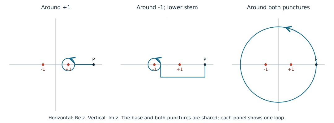
Specify loops before naming matrices

Take $P=3$ and small-circle radius $r=1/2$ by default. Every circle runs counterclockwise. A stem is the approach from the base to a circle, followed in reverse after that circle.

Loop	Actual path in the dimensionless plane
Plus	Real stem $P\to1+r$, circle centered at $+1$ of radius $r$, return along the stem
Minus	Broken stem $P\to P-i\to-1+r-i\to-1+r$, circle centered at $-1$, reverse stem
Outer	Circle centered at $0$ of radius $P$, starting and ending at $P$

The minus stem passes below the plus puncture. Changing its approach can conjugate the based monodromy; a matrix without this path specification is ambiguous. The program uses 64 straight chords per circle. Those polygons stay away from the punctures and have the same winding and homotopy as the circles for the accepted radii. This is an exact topological replacement, not an approximation to a path-dependent observable.

The red dots are excluded singularities. Each stem is traversed outward and back; the arrow on each circle fixes its orientation. The same path generator supplies the figure and the numerical continuation.

For this basis and these loops, the analytic targets are

$$M_+=\begin{pmatrix}1&0\\-2&1\end{pmatrix},\qquad M_-=\begin{pmatrix}-1&2\\-2&3\end{pmatrix},\qquad M_\infty=\begin{pmatrix}-1&2\\0&-1\end{pmatrix}. \tag{LAB14.2}$$

They are the matrices in Seiberg–Witten (5.3), (5.12)–(5.13), with the rooted paths made explicit here. Their analytic checks are different from numerical propagation. Near $+1$, write $b=a_D$. The logarithmic contribution $a\supset(i/\pi)b\log(b/\mu)$ changes by $-2b$ when $b$ winds once; analytic terms return unchanged. At large $u$, continuing $\sqrt u$ and its accompanying logarithm yields the outer matrix. The rooted relation then fixes the minus matrix.

Continue the differential equation

Both dimensionless periods obey

$$(z^2-1)p''+\frac14p=0. \tag{LAB14.3}$$

The canonical derivation is in the period lesson; Bilal (6.4), (6.11) provides a source check of its sign and coefficient. Expand about a regular point $z_0$: $p(z_0+h)=\sum_{n=0}^q c_nh^n$. Multiplying the series for $p''$ by $(z_0+h)^2-1$ and matching powers gives

$$c_{n+2}=-\frac{2z_0n(n+1)c_{n+1}+ \left[n(n-1)+\frac14\right]c_n} {(z_0^2-1)(n+2)(n+1)}. \tag{LAB14.4}$$

Start with $c_0=p(z_0)$ and $c_1=p'(z_0)$. Evaluate the polynomial and its derivative at the next point, then make those the new initial data. Each step has length at most $\eta\min(|z_0-1|,|z_0+1|)$, strictly within the nearest singularity. The code compares $(q,\eta)=(40,0.2)$ and $(60,0.1)$. The path is held fixed while the approximation inside each disk changes.

It is tempting to recover a matrix from the final values $D,A$ alone. Two equations would leave four unknown entries. Use their derivatives too. Define the fundamental matrix with solutions in columns:

$$F=\begin{pmatrix}D&A\\D'&A'\end{pmatrix},\qquad F_{\rm end}=F_{\rm start}M^T,\qquad M=(F_{\rm start}^{-1}F_{\rm end})^T. \tag{LAB14.5}$$

The transpose follows because $\Pi$ has solutions in a column, whereas $F$ stores each solution and derivative in a column. Omitting it changes which cycle is claimed invariant. The Wronskian $AD'-DA'=2i/\pi$ makes $F$ invertible. Its derivative vanishes by (LAB14.3), so it also tests propagation along the entire path. Only after comparing the complex entries with the analytic target does the program display a rounded integer matrix. Nearness to some integer matrix is an inadequate check: an accidental branch reset gives the integer identity.

The implementation also continues an already continued germ around a second loop. In the convention of the monodromy lesson, chronological plus then minus gives

$$\mathcal C_-(\mathcal C_+\Pi) =\mathcal C_-(M_+\Pi)=M_+M_-\Pi=M_\infty\Pi. \tag{LAB14.6}$$

Here $\mathcal C$ continues functions and leaves constant coefficients unchanged. This explains the order; it is not a rule to reverse ordinary matrix multiplication on vectors. Reversing the chronological loops yields $M_-M_+$ instead. The program checks both compositions and the inverse matrix from reversing the plus path.

Run and inspect a reproducible calculation

Download the complete lab (ZIP) with the program, pinned dependencies, reference output and run instructions.

Save these four files together: Python program, pinned requirement, baseline JSON and loop figure. With Python 3 and a local virtual environment, install the requirement using python -m pip install -r requirements.txt, then run:

python sw_monodromy.py
python sw_monodromy.py --base 4 --radius 0.35 --dps 70
python sw_monodromy.py --reset-branches
python sw_monodromy.py --figure loops.svg

There are no site imports, network requests or hidden data. Only the explicit --figure option writes a file. The permitted range is $2\le P\le6$, $0.15\le r\le0.7$ and 40–90 working decimal digits. The chosen ranges keep the stems and circles separated from both punctures; precision is not permission to cross a singularity.

At the default base, $A=2.43201344685$, $D=0.90649391984633i$ and $D'/A'=i$. The maximum entry residuals against (LAB14.2) are:

Loop	Order 40, disk fraction 0.2	Order 60, disk fraction 0.1
Plus	$1.88\times10^{-29}$	$6.62\times10^{-51}$
Minus with lower stem	$2.23\times10^{-29}$	$3.08\times10^{-50}$
Outer	$1.02\times10^{-35}$	$2.05\times10^{-50}$

The acceptance threshold is $10^{-24}$; determinant and Wronskian residuals are also printed. A separate twenty-digit precision repeat is applied to the plus loop. Refinement tests series truncation, while the precision repeat probes rounding. Neither is a certified interval bound. Positive $\operatorname{Im}\tau$ is checked at sampled propagation points; the finite sample is not an independent proof of positivity everywhere. Last reported digits can vary with arithmetic implementations.

The --reset-branches mode keeps the correctly continued values for comparison, but intentionally substitutes the original germ when computing the reported endpoint matrix. All three reported matrices become the identity and all three benchmark tests fail. intentional_branch_reset_detected becomes true. This demonstrates why feeding the same coordinate into a principal-branch library cannot measure monodromy.

Charge labels, couplings and the metric

For a passive change of frame $\Pi'=M\Pi$, describing the same charge requires

$$\gamma'=\gamma M^{-1},\qquad \gamma'\Pi'=\gamma\Pi. \tag{LAB14.7}$$

For the plus loop and initial row $(0,1)$, the new row is $(2,1)$. The default numbers make the check concrete: $D$ returns unchanged, $A$ becomes $A-2D$, and $2D+(A-2D)=A$. Keeping the original row $(0,1)$ instead gives $Z/\Lambda=A-2D=2.43201344685-1.8129878396927i$. That is continuation of a fixed row’s central-charge function, not the passive relabeling just performed.

Write $M=\left(\begin{smallmatrix}\alpha&\beta\\c&d\end{smallmatrix}\right)$. Derivatives transform by the same matrix, so

$$\tau'=\frac{\alpha\tau+\beta}{c\tau+d},\qquad \operatorname{Im}\tau'=\frac{\operatorname{Im}\tau}{|c\tau+d|^2},\qquad \operatorname{Im}\tau'|A'_{\rm new}|^2 =\operatorname{Im}\tau|A'_{\rm old}|^2. \tag{LAB14.8}$$

The middle identity follows by subtracting the complex conjugate and using $\det M=1$; $A'_{\rm new}=(c\tau+d)A'_{\rm old}$ proves the last identity. At $P=3$, the plus transformation takes $\tau=i$ to $(-2+i)/5$. The imaginary part changes, but the metric does not. This is a useful check that the derivative ratio, coordinate units and matrix order have been used together consistently.

The primitive invariant charge rows satisfy $\gamma M=\gamma$: $(1,0)$ for the plus matrix and $(1,-1)$ for the chosen minus matrix. These match the vanishing-cycle interpretation in Bilal (5.14)–(5.15). Multiples of an invariant row remain invariant algebraically. The computation cannot decide whether those multiples are single particles, multiparticle thresholds, or absent. Follow the stability lesson before interpreting a charge orbit as a spectrum.

Exercises

1. Reverse the order

Compute the result of continuing first around minus and then plus. Explain why it differs from the outer loop and find the matrix for the plus loop traversed twice clockwise.

Hint 1

Continue the coefficients of an already continued germ as constants, as in (LAB14.6).

Hint 2

For the last question write $M_+=I+N$ and calculate $N^2$.

Solution

The chronological minus-then-plus result is $M_-M_+=\left(\begin{smallmatrix}-5&2\\-8&3\end{smallmatrix}\right)$. Its difference from $M_+M_-$ is $\left(\begin{smallmatrix}-4&0\\-8&4\end{smallmatrix}\right)$, so order changes the based loop class seen by these germs. Both products have determinant1; that check alone cannot distinguish them. For $N=\left(\begin{smallmatrix}0&0\\-2&0\end{smallmatrix}\right)$ we have $N^2=0$, hence $M_+^{-2}=I-2N=\left(\begin{smallmatrix}1&0\\4&1\end{smallmatrix}\right)$. The sign and factor distinguish two clockwise windings from one counterclockwise winding. The program’s opposite-order and reversed-path residuals check the corresponding numerical operations separately.

2. Transform a charge and its coupling

At the default base use the initial row $(1,1)$ and the minus matrix. Find its passive row and its continued fixed-row central charge in terms of the initial $D,A$. Determine the transformed coupling and verify the metric factor.

Hint 1

The inverse matrix belongs in the passive charge transformation; the matrix itself belongs in the period transformation.

Hint 2

Here $c=-2$, $d=3$, and the initial coupling is $i$.

Solution

$M_-^{-1}=\left(\begin{smallmatrix}3&-2\\2&-1\end{smallmatrix}\right)$, so the passive row is $(5,-3)$. Since $D_{\rm new}=-D+2A$ and $A_{\rm new}=-2D+3A$, its central charge is $\Lambda[5(-D+2A)-3(-2D+3A)]=\Lambda(D+A)$, as required. Continuing the fixed row $(1,1)$ gives $\Lambda(-3D+5A)$ instead. The coupling is $(2-i)/(3-2i)=(8+i)/13$, whose imaginary part is $1/13$. Meanwhile $|A'_{\rm new}|^2=|3-2i|^2|A'|^2=13|A'|^2$. Their product is unchanged. The conserved quantity refers to the same physical charge or metric, not separately to each coordinate expression.

3. Change the circle without changing the question

Run the changed-base/radius command above. Predict the three matrices and invariant primitive rows. Does invariance of $(2,-2)$ under the minus matrix establish a stable particle with that charge? Explain which modifications of the loop could actually change the matrix.

Hint 1

Move the base along the real ray and deform the stems continuously, avoiding both punctures throughout.

Hint 2

The equation $\gamma M=\gamma$ is linear. Existence and stability of particles are additional physical questions.

Solution

Transporting the initial frame along the real ray and reducing the radii without crossing a puncture preserves the based loop classes and their matrices (LAB14.2). The rows remain $(1,0)$ and $(1,-1)$ up to an overall sign. The period values and the number of numerical steps change; the integer targets do not. $(2,-2)=2(1,-1)$ is invariant by linearity, but that fact supplies no bound state or stability argument. An extra winding changes a matrix power; reversing a loop inverts it; changing an approach so it winds around another puncture conjugates the based generator. A path through a puncture is inadmissible for this continuation. The matrix comparison should reject a changed path class unless its target is changed consistently.

The next useful question is physical: which charge combinations remain stable as the vacuum moves? Return to the central-charge and decay analysis with the period branches and charge frame now under control.