Higgs and Coulomb branches in 3D SQED

A potential can have a continuous family of zero-energy configurations. Before calling that family a space of vacua, we must identify configurations related by gauge transformations and decide which fields remain light. In three dimensions there is an additional step: a massless photon has one propagating polarization, which can be described locally by a periodic scalar.

We will carry out all three steps for the Abelian gauge theory just constructed. The other prerequisite is connections, flux, and holonomy, particularly its unit-charge flux convention.

The model remains three-dimensional $\mathcal N=2$ SQED, with four real Lorentzian supercharges, compact gauge group $U(1)$, one pair of chiral multiplets of charges $+1,-1$, gauge Chern–Simons level $k=0$, and zero superpotential, masses, and FI parameter. The coupling $g_{\rm YM}^2$ has dimension one. Background sources are zero, and we retain the paired regulator convention already specified. The matter scalars are $\phi_+,\phi_-$. They are two independent complex fields, not conjugates of one another.

First calculation: solve and identify the vacua

On the physical bosonic contour, the potential is

$$U=\sigma^2\bigl(|\phi_+|^2+|\phi_-|^2\bigr) +\frac{g_{\rm YM}^2}{2} \bigl(|\phi_+|^2-|\phi_-|^2\bigr)^2.$$

Here $\sigma$ is the real scalar in the vector multiplet. A translation-invariant vacuum has zero field strength, zero gradients, vanishing fermions and auxiliaries, and $U=0$. Positivity gives

$$\sigma\phi_+=\sigma\phi_-=0,\qquad |\phi_+|=|\phi_-|.$$

There are two possibilities:

Solutions	Gauge symmetry and light fields
$\sigma=0$, $\lvert\phi_+\rvert=\lvert\phi_-\rvert=v>0$	The gauge field becomes massive; a gauge-invariant matter modulus remains.
$\phi_+=\phi_-=0$, $\sigma$ arbitrary	The $U(1)$ gauge symmetry remains unbroken; the photon and $\sigma$ remain massless at tree level.

The first family, including its endpoint $v=0$, is the Higgs branch. The second is the Coulomb branch. These names refer to which fields describe the low-energy motion along the family. There is no mixed branch with both $\sigma\ne0$ and nonzero matter in this rank-one model. A zero-energy member preserves all four flat-space supercharges.

For the Higgs solutions, write

$$\phi_+=v e^{i\alpha_+},\qquad \phi_-=v e^{i\alpha_-}.$$

A gauge transformation acts as $\alpha_+\mapsto\alpha_++\lambda$, $\alpha_-\mapsto\alpha_--\lambda$. The sum $\theta=\alpha_++\alpha_-$ survives and has period $2\pi$. Thus the invariant complex coordinate is

$$\boxed{M=\phi_+\phi_-=v^2e^{i\theta}.}$$

It is called the meson, meaning this neutral matter composite. Every complex value occurs: for $M\ne0$, choose $\phi_-=\sqrt{|M|}$ and $\phi_+=M/\sqrt{|M|}$. Conversely, equal $M$ and equal magnitudes determine the same gauge orbit. At $M=0$, the equal-magnitude condition forces both fields to vanish.

The quotient therefore has one complex dimension and is $\mathbb C$ as a complex algebraic space. One can also check its coordinate functions: a holomorphic monomial $\phi_+^a\phi_-^b$ is gauge invariant precisely when $a=b$, so every invariant polynomial is a polynomial in $M$. This argument does not claim that its kinetic metric is the ordinary flat metric of the $M$ plane.

Counting gives the same result away from the origin: four real matter components, minus one real constraint, minus one gauge-orbit direction, leaves two real coordinates. At the origin the gauge orbit shrinks to a point, so that regular counting argument alone cannot determine the local metric.

The Higgs metric comes from minimizing gauge motion

Consider slowly varying Higgs coordinates at $v>0$. The scalar kinetic term is

$$|(\partial_\mu-ia_\mu)\phi_+|^2 +|(\partial_\mu+ia_\mu)\phi_-|^2 =2(\partial_\mu v)^2 +v^2\bigl[(\partial_\mu\alpha_+-a_\mu)^2 +(\partial_\mu\alpha_-+a_\mu)^2\bigr].$$

At leading order in derivatives, eliminate the massive connection by minimizing this expression:

$$a_\mu=\frac12\partial_\mu(\alpha_+-\alpha_-),\qquad \mathcal L_{\rm Higgs}^{(2)} =2(\partial v)^2+\frac{v^2}{2}(\partial\theta)^2 =\frac{\partial_\mu M\,\partial^\mu\overline M}{2|M|}.$$

The Maxwell term contributes at higher derivative order in this elimination. The two-derivative coefficient is also obtained from the Kähler potential $K=2\sqrt{M\overline M}$: $\partial_M\partial_{\overline M}K=1/(2|M|)$. Here “Kähler potential” means a function whose mixed derivative supplies the complex scalar kinetic coefficient.

For clarity, define the metric convention by $\mathcal L^{(2)}=G_{M\overline M}\partial M\partial\overline M$ and $d\ell_H^2=G_{M\overline M}dM\,d\overline M$. Setting $\rho=\sqrt2v$ gives

$$d\ell_H^2=d\rho^2+\frac{\rho^2}{4}d\theta^2,\qquad \theta\sim\theta+2\pi.$$

A circle at radial distance $\rho$ has circumference $\pi\rho$, rather than $2\pi\rho$. This is a cone of opening angle $\pi$. Its conical metric and its complex coordinate $M\in\mathbb C$ describe different features of the same tree-level quotient. There is no unbroken $\mathbb Z_2$ gauge group at $v>0$: a charge-one nonzero expectation value is fixed only by the identity of $U(1)$.

This is a tree-level low-energy metric. The vector mass is $m_V=2g_{\rm YM}v$, with $g_{\rm YM}>0$ the square root of $g_{\rm YM}^2$. Eliminating it requires momenta $E\ll m_V$; the weakly coupled Higgs regime is $v\gg g_{\rm YM}$. The limit $v\to0$ removes both controls. The cone does not establish the exact quantum metric at its tip.

A Coulomb patch contains a compact scalar

Set $\phi_\pm=0$ and choose a constant $\sigma_0\ne0$. Charged matter has mass magnitude $|\sigma_0|$. Its two fermion mass signs are opposite, so their induced gauge Chern–Simons levels cancel in the specified convention. There is consequently a massless Maxwell field in this patch.

We first keep the tree-level terms,

$$\mathcal L_{\rm Coulomb,E} =\frac1{4g_{\rm YM}^2}f_{\mu\nu}f_{\mu\nu} +\frac1{2g_{\rm YM}^2}(\partial_\mu\sigma)^2, \qquad f_{\mu\nu}=\partial_\mu a_\nu-\partial_\nu a_\mu.$$

This approximation requires $E\ll|\sigma_0|$ and $|\sigma_0|\gg g_{\rm YM}^2$. The first condition permits removal of charged matter; the second suppresses quantum corrections relative to the tree kinetic terms. The gauge group is already Abelian, so $\sigma\ne0$ does not break it further. In particular, no Weyl identification equates $\sigma$ and $-\sigma$.

In oriented Euclidean Cartesian coordinates, define

$$b^\mu=\frac12\epsilon^{\mu\nu\rho}f_{\nu\rho}, \qquad \epsilon^{123}=1.$$

Then $f_{\mu\nu}f_{\mu\nu}=2b_\mu b_\mu$, and the Bianchi identity $df=0$ is $\partial_\mu b^\mu=0$. Introduce a dimensionless scalar $\gamma$ as a multiplier for this identity:

$$S_{\rm first} =\int d^3x\,\frac{b^2}{2g_{\rm YM}^2} +\frac{i}{2\pi}\int\gamma\,df.$$

Here $f=\tfrac12f_{\mu\nu}dx^\mu\wedge dx^\nu$. The local calculation treats its three components as independent. Global flux sectors must still be retained; a local multiplier equation alone does not impose integral flux.

After integration by parts, with its surface term absent,

$$\mathcal L_{\rm first} =\frac{b^2}{2g_{\rm YM}^2} -\frac{i}{2\pi}b^\mu\partial_\mu\gamma =\frac1{2g_{\rm YM}^2} \left(b-\frac{i g_{\rm YM}^2}{2\pi}d\gamma\right)^2 +\frac{g_{\rm YM}^2}{8\pi^2}(d\gamma)^2.$$

Integrating the Gaussian over real $b$ therefore gives the positive scalar action

$$\boxed{\mathcal L_{\rm dual,E} =\frac{(\partial\sigma)^2}{2g_{\rm YM}^2} +\frac{g_{\rm YM}^2}{8\pi^2}(\partial\gamma)^2.}$$

Its saddle is $b=i g_{\rm YM}^2d\gamma/(2\pi)$. The factor $i$ belongs to Euclidean dualization: it is a complex Gaussian saddle, not an equality between real classical configurations on the two Euclidean contours. Omitting it would give a negative scalar kinetic term.

This scalar replaces the photon polarization; it does not add another propagating degree of freedom. Together $\sigma$ and $\gamma$ provide the two real bosonic modes of the original vector multiplet. The periodic scalar description and its supersymmetric organization are discussed in AHISS v1, §§2.2–2.3, printed pages 5–6.

Fix the period by matching magnetic charge

The unit-charge gauge convention fixes

$$\frac1{2\pi}\int_{\Sigma_2}f\in\mathbb Z.$$

The corresponding normalized topological current is

$$j_J^\mu=\frac1{4\pi}\epsilon^{\mu\nu\rho}f_{\nu\rho}.$$

Its conservation follows from the Bianchi identity, without using the Maxwell equation. It is a global current, not the electric gauge current. We consider the continuum theory with this topological symmetry and no added interaction that violates it.

To identify its generator, return temporarily to Lorentzian signature $(+--)$, with $\epsilon^{012}=1$. The continuation of the dual action has positive time kinetic terms. In our orientation its magnetic relation is

$$B=f_{12}=\frac{g_{\rm YM}^2}{2\pi}\dot\gamma,\qquad \pi_\gamma=\frac{g_{\rm YM}^2}{4\pi^2}\dot\gamma =\frac{B}{2\pi}=j_J^0.$$

Thus the total magnetic charge generates shifts of $\gamma$. On a compact spatial surface its allowed values are integers. A coordinate with conjugate momenta $n\in\mathbb Z$ is an angle of period $2\pi$:

$$\boxed{\gamma\sim\gamma+2\pi.}$$

Equivalently, its zero-mode wavefunctions are $e^{in\gamma}$. Choosing a different period while keeping the current and the allowed unit flux fixed would change the theory.

At tree level the natural dimensionless complex coordinate is

$$u=\frac{2\pi\sigma}{g_{\rm YM}^2}+i\gamma,\qquad \mathcal L_{\rm dual,E} =\frac{g_{\rm YM}^2}{8\pi^2}\partial_\mu u\,\partial_\mu\overline u, \qquad u\sim u+2\pi i.$$

The formal free-photon target is a cylinder. The exponential $w=e^u$ is single-valued on that cylinder and never vanishes there. These statements concern a local semiclassical description. They do not identify $w$ with a globally defined quantum operator at the massless-matter point.

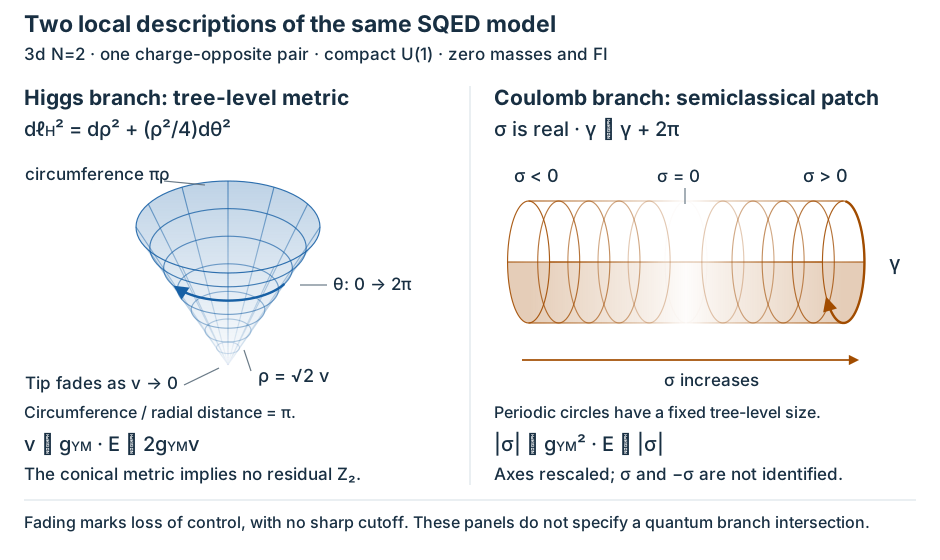
The left surface realizes $d\ell_H^2=d\rho^2+\rho^2d\theta^2/4$, with $\rho=\sqrt2v$ and $\theta$ of period $2\pi$. Its smaller circumference does not imply a residual discrete gauge group. The right cylinder has the independent angle $\gamma\sim\gamma+2\pi$ and is drawn with rescaled axes. Use the Higgs description for $v\gg g_{\rm YM}$ and $E\ll2g_{\rm YM}v$, and the Coulomb description for $|\sigma|\gg g_{\rm YM}^2$ and $E\ll|\sigma|$. Fading indicates loss of these controls without assigning a sharp cutoff. Neither panel supplies the quantum geometry or a rule for joining the branches.

Worked check: magnetic flux is a rotor momentum

Place the low-energy theory on a large flat spatial two-torus of area $\mathcal A$, with $\sigma$ fixed far along a Coulomb patch. This is a normalization check using excited flux sectors, not a claim of extra zero-energy vacua. In sector $n$, a uniform magnetic field minimizes the Maxwell energy:

$$B_n=\frac{2\pi n}{\mathcal A},\qquad E_n=\frac{\mathcal A}{2g_{\rm YM}^2}B_n^2 =\frac{2\pi^2n^2}{g_{\rm YM}^2\mathcal A}.$$

For the spatially constant dual photon,

$$L_0=\frac{\mathcal A g_{\rm YM}^2}{8\pi^2}\dot\gamma_0^2 =\frac I2\dot\gamma_0^2,\qquad I=\frac{\mathcal A g_{\rm YM}^2}{4\pi^2}.$$

An angular coordinate of period $2\pi$ has momentum $n$, so its rotor energy is $n^2/(2I)$, exactly the Maxwell result. It vanishes only for $n=0$. The equality tests both the kinetic coefficient and the period.

The derivative expansion additionally requires weak flux, $|B_n|\ll\sigma_0^2$, and energies and inverse torus lengths below $|\sigma_0|$. One can satisfy these conditions for any fixed $n$ by taking a sufficiently large torus. This is not an unrestricted claim about arbitrarily large flux density.

What the classical coordinates do not determine

The scalar potential sees the real coordinate $\sigma$, while the dual photon comes from the massless gauge field. Extending the free-photon cylinder through $\sigma=0$ would discard charged fields precisely where their mass vanishes. Likewise, extending the Higgs sigma model to $M=0$ discards a vector multiplet precisely where its mass vanishes. Neither extension is a controlled description of the intersection.

Even before asking about that point, quantum corrections can change the relation between $\sigma$ and a complex Coulomb coordinate. For example, suppose the two-derivative Abelian action in a regular patch has a positive coefficient $h(\sigma)$:

$$\mathcal L_E=\frac{h(\sigma)}4f^2 +\frac{h(\sigma)}2(\partial\sigma)^2.$$

The same Gaussian calculation gives

$$\mathcal L_{\rm dual,E} =\frac{h(\sigma)}2(\partial\sigma)^2 +\frac1{8\pi^2h(\sigma)}(\partial\gamma)^2.$$

Define $x$ locally by $dx/d\sigma=2\pi h(\sigma)$. Then

$$\mathcal L_{\rm dual,E} =\frac1{8\pi^2h(\sigma)} \left[(\partial x)^2+(\partial\gamma)^2\right].$$

The local complex coordinate is now $x+i\gamma$; it reduces to $u$ only for $h=1/g_{\rm YM}^2$. This is a conditional calculation for a given effective kinetic function, not a computation of that function for SQED.

For this SQED theory, the quantum description has two Coulomb components meeting the Higgs component at a common point; the classical cylinder is not the global answer. AHISS v1, §3.1, printed pages 12–14 develops that result. Its global operator interpretation requires additional input. The infrared-duality setting is also explained in Willett and Yaakov v2, §3, printed pages 6–8; an infrared duality does not assert equality of the tree-level metrics throughout the ultraviolet field space.

In particular, the identity $e^u e^{-u}=1$ in one cylinder chart cannot be promoted to a relation between globally continued quantum Coulomb operators on different components.

Exercises

1. An orbit, a coordinate, and a metric

Consider the Higgs representatives $(\phi_+,\phi_-)=(v e^{i\beta},v)$ and $(v,v e^{i\beta})$, with $v>0$. Find the gauge transformation relating them and their common $M$. Then compute the length of the circle $|M|=v^2$ using the quotient metric. Does the cone angle imply an unbroken discrete gauge group?

First hint

A gauge transformation changes the two phases with opposite signs. Their sum is unchanged.

Second hint

For fixed $v$, the metric is $v^2d\theta^2/2$, and the radial distance from the tip is $\rho=\sqrt2v$.

Solution

Choose $\lambda=-\beta$. It sends $(v e^{i\beta},v)$ to $(v,v e^{i\beta})$, and both have $M=v^2e^{i\beta}$. The circle length is

$$L=\int_0^{2\pi}\frac v{\sqrt2}\,d\theta =\sqrt2\pi v=\pi\rho.$$

This is the angle-$\pi$ cone metric, even though $M$ runs over a complex plane. At either nonzero representative, a transformation fixing $\phi_+$ requires $e^{i\lambda}=1$, so its stabilizer is trivial. In particular $\lambda=\pi$ changes both fields’ signs and does not fix that representative. It relates gauge-equivalent representatives; it is not an unbroken $\mathbb Z_2$ subgroup.

2. Rescale the angle without changing the theory

Define the dimensionful dual scalar $\chi=g_{\rm YM}^2\gamma/(2\pi)$. Find its period and kinetic term, then find a canonically normalized real scalar $\varphi_c$ with Lagrangian $(\partial\varphi_c)^2/2$. What is the circumference of its field-space circle? Finally, diagnose a Euclidean first-order calculation that replaces $-i b\cdot d\gamma/(2\pi)$ by $-b\cdot d\gamma/(2\pi)$.

First hint

Transform the period and the derivative coefficient together. Here the coupling is constant.

Second hint

Complete the square again with a real, rather than imaginary, linear coefficient.

Solution

The period becomes $\chi\sim\chi+g_{\rm YM}^2$, and

$$\mathcal L_\chi=\frac{(\partial\chi)^2}{2g_{\rm YM}^2}, \qquad \varphi_c=\frac{\chi}{g_{\rm YM}} =\frac{g_{\rm YM}\gamma}{2\pi}, \qquad \varphi_c\sim\varphi_c+g_{\rm YM}.$$

Its circumference is $g_{\rm YM}$ and its radius is $g_{\rm YM}/(2\pi)$. This circle is in scalar field space, so its circumference has the scalar’s mass dimension $1/2$; it is not a spatial length. The dimensions of $\chi$ and $\gamma$ are one and zero, respectively.

With the incorrect real Euclidean multiplier,

$$\frac{b^2}{2g_{\rm YM}^2}-\frac{b\cdot d\gamma}{2\pi} =\frac{(b-g_{\rm YM}^2d\gamma/(2\pi))^2}{2g_{\rm YM}^2} -\frac{g_{\rm YM}^2}{8\pi^2}(d\gamma)^2.$$

The resulting scalar action has the wrong sign. The imaginary Fourier multiplier in the Euclidean path integral is essential. A real Lorentzian duality relation does not justify deleting that factor before analytic continuation.

3. A corrected kinetic function is not an exact geometry

On a positive-$\sigma$ patch, consider the illustrative function

$$h(\sigma)=\frac1{g_{\rm YM}^2}+\frac c\sigma,\qquad c>0.$$

Here $c$ is a dimensionless model coefficient, not a claimed exact SQED loop coefficient. Obtain $x(\sigma)$, with a dimensionful reference scale $\sigma_*>0$ in any logarithm, and the dual angular kinetic coefficient. Does using this expression all the way to $\sigma=0$ prove the quantum branch intersection?

First hint

Integrate $dx/d\sigma=2\pi h(\sigma)$. A logarithm requires a dimensionless argument.

Second hint

The angular coefficient is the inverse of $h$, up to $8\pi^2$. Separately examine the mass of the charged fields removed from the patch.

Solution

Up to an additive constant,

$$x(\sigma)=\frac{2\pi\sigma}{g_{\rm YM}^2} +2\pi c\log\frac{\sigma}{\sigma_*}, \qquad G_{\gamma\gamma}^{(\mathcal L)} =\frac{g_{\rm YM}^2\sigma} {8\pi^2(\sigma+c g_{\rm YM}^2)}.$$

Both $x$ and $\gamma$ are dimensionless. At $\sigma\gg c g_{\rm YM}^2$, the angular coefficient approaches its tree value. The logarithmic correction changes the real part of the complex coordinate, so merely keeping $2\pi\sigma/g_{\rm YM}^2+i\gamma$ would miss it.

If extrapolated formally, the angular coefficient tends to zero as $\sigma\to0$. That observation alone does not prove the quantum geometry: the ansatz was not derived as an exact kinetic function, and charged matter becomes massless at the endpoint. Its removal requires $E\ll|\sigma|$, while a perturbative treatment of the original model also fails when $|\sigma|$ is comparable to $g_{\rm YM}^2$. Additional light fields and global operator relations are needed to decide how the components meet.

You should now be able to derive both the Higgs quotient and the normalized local Coulomb cylinder, and to name the mass scale that limits each effective description. Define and charge the simplest monopole operators constructs a local flux insertion and calculates its quantum charges. Those data supply information that the classical coordinates cannot.