Riemann surfaces from square roots: cuts and cycles

Monodromy showed that electric and magnetic periods change together when a vacuum travels around a singularity. We now need a geometric object on which that mixing has a visible meaning. Two sheets of a square root will supply it.

No complex-curve background is assumed. The variables in the mathematical examples below are dimensionless and are not yet the physical $u,a,a_D$. The application remains the rank-one Coulomb branch of four-dimensional N=2 $SU(2)$ theory, with eight real supercharges. The surface we construct is auxiliary geometry, not physical spacetime.

A square root becomes a single-valued coordinate

Consider

$$y^2=P(x),\qquad P(x)=\prod_{j=1}^4(x-e_j), \tag{SW09.1}$$

with distinct complex numbers $e_j$. At a generic $x$, there are two points on the surface, $(x,+\sqrt{P(x)})$ and $(x,-\sqrt{P(x)})$. A sheet is a local choice between them. The full pair $(x,y)$, rather than $x$ alone, tells us where we are.

Why call this a curve and a surface? One complex equation in two complex variables leaves one complex coordinate locally: a complex curve. One complex coordinate is two real coordinates: a real surface. A Riemann surface is such a surface with compatible holomorphic coordinates.

Near a simple zero $e$, write $P(x)=(x-e)G(x)$ with $G(e)\ne0$. Introduce a coordinate $s$ by

$$x=e+s^2,\qquad y=s\sqrt{G(e+s^2)}. \tag{SW09.2}$$

The remaining square root is single-valued in a sufficiently small disk. The surface is smooth at $s=0$. What fails there is using $x$ as a coordinate: $dx/ds=0$. Thus $x=e$ is a branch point of the projection to the $x$ plane, not a singular point of the smooth surface.

One turn around $e$ sends $s\mapsto-s$, so a lifted path ends on the opposite sheet. Two turns return it to its starting point. A loop in the $x$ plane is therefore not automatically a closed loop on the surface.

Glue the sheets and include infinity

For a drawing, put the four roots on the real axis in the order $e_1<e_2<e_3<e_4$. Make cuts along $[e_1,e_2]$ and $[e_3,e_4]$. On each of two copies of the cut plane, choose a square-root branch. Glue the upper bank of each cut on one sheet to the lower bank on the other, and vice versa. This cross-gluing makes $y$ continuous when a path crosses a seam.

The cuts are not boundaries of the completed surface. Their positions are choices used to display it. Dragging a cut without moving its endpoints or crossing other marked data changes the drawing, not the surface.

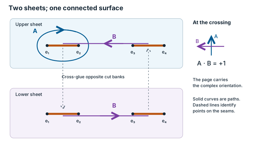
Solid blue is $A$ on the upper sheet. Purple is $B$, going from the right slit to the left slit on that sheet and returning on the lower one. Dashed vertical connectors mark identified seam points, not extra pieces of the surface. A small separation of coincident cut banks is understood. The arrows give $A\cdot B=+1$ with the usual complex orientation.

To discuss a compact surface, infinity must be included. Set $z=1/x$ and $Y=yz^2$. Equation (SW09.1) becomes

$$Y^2=\prod_{j=1}^4(1-e_jz). \tag{SW09.3}$$

At $z=0$, there are two distinct smooth points, $Y=+1$ and $Y=-1$. Infinity is not a branch point for this quartic. We have a degree-two map from the compact surface to the $x$ sphere, with precisely four simple branch points.

Count its topology by triangulating that sphere with all branch points among its vertices. If the base has $V,E,F$ cells, each edge and face has two lifts. An ordinary vertex has two lifts, but a branch vertex has one. With $b$ simple branch points,

$$\chi_{\rm cover}=(2V-b)-2E+2F =2\chi_{\rm sphere}-b=4-b. \tag{SW09.4}$$

For $b=4$, this is zero. A connected compact oriented surface of genus $g$ has $\chi=2-2g$, so $g=1$: a torus, meaning a surface with one handle. This is a topological statement; it does not give a preferred circular doughnut shape or a metric.

The double-cover construction and genus-one interpretation are the ingredients used in Seiberg–Witten, (6.6)–(6.9). Its cubic presentation has a fourth branch point at infinity; Exercise 1 checks that difference.

Closed curves, orientation, and intersection

An oriented closed path is a cycle. For present purposes we identify cycles if their difference bounds a region of the surface. This is homology: it remembers winding around a handle while discarding small contractible detours. Reversing a cycle gives its negative.

On our torus, the depicted cycles $A$ and $B$ generate the closed-curve homology. Any class is $mA+nB$ with integers $m,n$. One can see the two generators by cutting the torus along them: the remaining polygon has four edges identified in pairs. A path’s net crossings of these identifications give its two winding numbers.

To define intersection, move curves slightly so they cross transversely rather than overlap. At a crossing, count $+1$ if the ordered tangent vectors of the first and second curve agree with the surface orientation, and $-1$ otherwise. Sum the signs. Our figure uses $A\cdot B=+1$, hence $B\cdot A=-1$, and

$$(mA+nB)\cdot(pA+qB)=mq-np. \tag{SW09.5}$$

The sign is part of the convention, not an absolute property of the letters $A,B$. These generic mathematical cycles have not yet been assigned to the physical electric and magnetic periods.

A differential is locally an expression such as $\omega=f(s)\,ds$ that transforms consistently between coordinate charts. For example,

$$\omega=\frac{dx}{y} =\frac{2\,ds}{\sqrt{G(e+s^2)}} \tag{SW09.6}$$

is finite at each simple branch point. For the quartic, it is $-dz/Y$ at either infinity and is finite there too. Apparent singularities of $dx/y$ in the $x$ description need not be actual poles on the surface.

The integral $P_A=\oint_A\omega$ is called a period. It is calculated along the entire lifted path, including sheet changes. For a holomorphic differential, Stokes’ theorem makes the integral depend only on the cycle’s homology class, so $P_{mA+nB}=mP_A+nP_B$. If the differential has poles, cycles may be deformed freely only while avoiding them; crossing a pole requires accounting for its residue.

An oriented basis change $(A',B')=(aA+bB,cA+dB)$ preserves $A'\cdot B'=1$ exactly when $ad-bc=1$. This is the geometric origin of integral determinant-one transformations of period pairs. Assigning a particular physical period requires a particular differential and basis in addition to this topology.

Work an integral through both sheets

The neighborhood of two approaching branch points can be modeled by

$$y^2=x^2-\delta^2,\qquad \delta>0. \tag{SW09.7}$$

This is a local neck model, not the full four-branch-point torus. A contour around the cut $[-\delta,\delta]$ can be shrunk onto its two banks. Parametrize the lifted contour by

$$x=\delta\cos\theta,\qquad y=i\delta\sin\theta,\qquad 0\leq\theta\leq2\pi. \tag{SW09.8}$$

For $0<\theta<\pi$, it travels from right to left on the bank with positive imaginary $y$; for $\pi<\theta<2\pi$, it returns on the other bank. At the endpoints, (SW09.2) supplies a regular coordinate. The apparent $0/0$ in the first integrand has a finite limit. Directly,

$$\oint_A\frac{dx}{y} =\int_0^{2\pi}i\,d\theta=2\pi i,\qquad \oint_A y\,dx =-i\delta^2\int_0^{2\pi}\sin^2\theta\,d\theta =-i\pi\delta^2. \tag{SW09.9}$$

Both integrals require the return sheet. Using the same sign of $y$ on both banks would incorrectly cancel them.

As $\delta\to0$, the cycle collapses onto the collision, but only the second integral vanishes. The first differential develops singular behavior in the limiting geometry. A shrinking cycle alone does not imply a vanishing period of every differential. This is precisely why choosing the Seiberg–Witten differential will be a separate physical step.

Move branch points and watch a cycle twist

We can derive the local cycle transport without a drawing of a complicated moving torus. In (SW09.7), set

$$v=x+y,\qquad w=x-y,\qquad vw=\delta^2=t. \tag{SW09.10}$$

For fixed small nonzero $t$, restrict to $|v|<R$ and $|w|<R$. The remaining region is the annulus $|t|/R<|v|<R$. Its middle circle is the cycle that will shrink when $t=0$.

Orient this circle $A$ by increasing $\arg v$. Orient a crossing curve $B$ inward, from the outer $v$ boundary toward the inner one, so that $A\cdot B=+1$. Keep its outer endpoint fixed in the $v$ chart and its other endpoint fixed in the $w$ chart. At the inner endpoint,

$$\arg v=\arg t-\arg w. \tag{SW09.11}$$

When $t$ goes counterclockwise once around zero, the inner endpoint’s continuously followed $v$ angle gains $2\pi$ relative to the outer endpoint. The crossing curve acquires one positive turn of the annulus. After attaching the unchanged outside part of the surface, this says

$$A\longmapsto A,\qquad B\longmapsto B+A. \tag{SW09.12}$$

This operation is a Dehn twist: cut along the annulus, turn one boundary once relative to the other, and glue it back. Equation (SW09.11) fixes the sign for our orientations.

There is an essential factor-of-two distinction. A single $t$ loop sends $\delta=\sqrt t$ to $-\delta$: it exchanges the two branch points. Returning each labeled root to itself by a full turn of their separation $\delta$ makes $t=\delta^2$ wind twice. It gives $B\mapsto B+2A$. Confusing exchange with full winding loses a factor two even before any physical normalization is considered.

Tachikawa, section 4.3.3, uses a branch-point exchange to calculate cycle transport. His physical curve and charge conventions differ from our first-paper package, so his numerical period matrix is not imported here. Our annulus argument is mathematical; the orientation and ordering of physical periods must still be specified. For example, the illustrative column $(P_A,-P_B)^T$ transforms under the full labeled-root winding by $\begin{pmatrix}1&0\\-2&1\end{pmatrix}$. This matches the form of the monopole shear, but does not yet identify these test periods with $a_D,a$.

At $t=0$, the local equation is $vw=0$, two branches crossing at a node. Unlike a simple branch point of the projection, this is an actual singularity of the surface. The smooth torus with a narrow neck has reached a degenerate limit.

Exercises

1. Find the missing branch point

Consider $y^2=(x-e_1)(x-e_2)(x-e_3)$ with distinct roots. Show that infinity is a branch point, count the genus, and check that $dx/y$ is regular there. Then determine the genus of a degree-five polynomial with distinct roots.

Hint 1

Use $z=1/x$ and $Y=yz^2$ for the cubic. Does $Y^2$ have a simple zero at $z=0$?

Hint 2

For the cubic, a uniform local coordinate is $s=1/\sqrt{x}$ rather than $1/x$. Count all branch points before using (SW09.4).

Solution

The cubic becomes $Y^2=z\prod_j(1-e_jz)$. Near $z=0$, the coordinate $Y$ is proportional to $\sqrt z$, so there is one ramified point above infinity. The three finite points and infinity give $b=4$, hence $\chi=0$ and $g=1$.

More explicitly, $x=s^{-2}$ and $y=s^{-3}\sqrt{\prod_j(1-e_js^2)}$. Therefore

$$\frac{dx}{y}=-\frac{2\,ds}{\sqrt{\prod_j(1-e_js^2)}},$$

which is regular at $s=0$. In the quintic, $Y=yz^3$ gives $Y^2=z\prod_{j=1}^5(1-e_jz)$. Infinity again branches, now giving $b=6$, $\chi=-2$, and $g=2$. Omitting infinity would give an impossible half-integer genus.

2. Why does the sphere example have a nonzero integral?

Compactify the two-branch model (SW09.7). It has genus zero by (SW09.4), so its closed curves are contractible on the compact smooth surface. Explain why $\oint dx/y=2\pi i$ does not contradict Stokes’ theorem. Use $v=x+y$ to locate the poles and check the sign of the integral.

Hint 1

Solve $v=x+y$, $x-y=\delta^2/v$ for $x,y$, then differentiate.

Hint 2

The compactified $v$ plane has points $v=0$ and $v=\infty$. A meromorphic differential can have poles at both.

Solution

Solving gives $x=(v+\delta^2/v)/2$ and $y=(v-\delta^2/v)/2$. Thus $dx/y=dv/v$. The local coordinate $v$ covers the compactified surface as a sphere. The differential has residue $+1$ at $v=0$ and residue $-1$ at infinity, as follows by writing $v=1/z$.

Our contour (SW09.8) has $v=\delta e^{i\theta}$, oriented counterclockwise. The residue theorem gives $+2\pi i$, agreeing with the direct two-bank calculation. Contracting it on the compact sphere sweeps across a pole, where the hypothesis for applying Stokes to a smooth differential fails. This example is not a holomorphic differential on a genus-zero compact surface.

3. Keep the labels, signs, and periods separate

In the annulus model, let the labeled separation follow $\delta(s)=\delta_0 e^{2\pi i s}$. Find the transport of $mA+nB$ and verify its intersection pairing with another transported cycle. Then suppose a differential has period column $(P_A,-P_B)^T$. Derive its matrix and explain why this calculation alone is not a proof that a physical particle becomes massless.

Hint 1

The annulus parameter is $t=\delta^2$, so count its winding rather than just the endpoint of $\delta$.

Hint 2

Use linearity of integration and compare $(m+2n)q-n(p+2q)$ with (SW09.5). Whether $P_A$ tends to zero depends on the differential.

Solution

There are two twists, so $mA+nB$ goes to $(m+2n)A+nB$. The other cycle $pA+qB$ goes to $(p+2q)A+qB$. Their intersection remains $(m+2n)q-n(p+2q)=mq-np$.

The periods satisfy $P_A'=P_A$, $P_B'=P_B+2P_A$, and hence

$$\begin{pmatrix}P_A'\\-P_B'\end{pmatrix} =\begin{pmatrix}1&0\\-2&1\end{pmatrix} \begin{pmatrix}P_A\\-P_B\end{pmatrix}.$$

For the local test differential $y\,dx$, (SW09.9) gives $P_A=-i\pi\delta^2\to0$; for $dx/y$, it stays $2\pi i$. Physical BPS masses require the correctly normalized physical differential and charge map, and the existence of the relevant state. Neither the drawing nor this determinant-one matrix establishes all of those inputs.

From geometry back to the gauge theory

A square-root equation now gives us a smooth surface, a calculable genus, oriented cycles and a way to follow them as parameters move. Choose the Seiberg–Witten curve and differential next fixes the physical normalization by matching weak-coupling behavior and the vanishing monopole period. That normalization is not fixed by the word “torus.”