A finite-dimensional localization example

An integral can change its appearance without changing its value. Supersymmetric localization makes this useful: deform the integrand until only a simple neighborhood contributes, and use a symmetry identity to show that the answer stayed fixed. The identity, its boundary assumptions and the fluctuation integral are all essential.

We will do the complete calculation for two ordinary variables and two Grassmann variables. The only preparation is Grassmann calculus. This is a zero-dimensional mathematical model, with dimensionless integration variables and one odd symmetry operation. It is not being assigned the spacetime supercharges or gauge group of a three- or four-dimensional field theory. Those theories will use the same reasoning with additional analytic requirements.

An odd operation whose square rotates

Let $x,y$ range over $\mathbb R$, and let $\psi_1,\psi_2$ be odd generators. Retain left derivatives and the ordered measure

$$\int d\psi_2\,d\psi_1\,\psi_1\psi_2=1.$$

Define an odd operation $Q$ by

$$Qx=\psi_1,\qquad Qy=\psi_2,\qquad Q\psi_1=y,\qquad Q\psi_2=-x, \tag{O01.1}$$

and extend it by the graded product rule $Q(AB)=(QA)B+(-1)^{|A|}A(QB)$. Equivalently,

$$Q=\psi_1\partial_x+\psi_2\partial_y +y\partial^L_{\psi_1}-x\partial^L_{\psi_2}.$$

Applying $Q$ twice gives

$$Q^2x=y,\quad Q^2y=-x,\quad Q^2\psi_1=\psi_2,\quad Q^2\psi_2=-\psi_1.$$

Thus $Q^2=J$, where $J$ generates simultaneous clockwise rotations of the two pairs. In particular, $Q$ is not nilpotent on every function. It squares to zero on rotation-invariant expressions.

A quantity $\mathcal O$ is Q-closed if $Q\mathcal O=0$. It is Q-exact if it can be written $\mathcal O=QV$. An exact expression is closed when $Q^2V=JV=0$. We must check this condition rather than infer it from the word “exact.” This is the algebraic pattern used in the general localization argument in Pestun’s introduction, version 3, pp. 5–6.

Set $\rho=x^2+y^2$ and choose the odd, rotation-invariant expression

$$V=y\psi_1-x\psi_2.$$

Its variation is especially useful:

$$QV=\rho-2\psi_1\psi_2. \tag{O01.2}$$

For example, $Q(y\psi_1)=\psi_2\psi_1+y^2$, so the Grassmann interchange supplies one of the two minus signs. Directly, $Q\rho=2(x\psi_1+y\psi_2)$ and $Q(\psi_1\psi_2)=x\psi_1+y\psi_2$; these terms cancel in $Q(QV)$.

Start with a non-Gaussian integral

Take a fixed real parameter $g\geq0$ and the even action

$$S_g=Q\bigl[(1+g\rho)V\bigr] =\rho+g\rho^2-2(1+2g\rho)\psi_1\psi_2. \tag{O01.3}$$

The preimage is rotation invariant, so $QS_g=0$. For $g>0$ the ordinary part has a quartic interaction in $x,y$. The accompanying Grassmann interaction is required by the symmetry.

Add $tQV$, with $t\geq0$, and write $a=1+t$. Our integral is

$$Z(t,g)=\frac1{2\pi} \int_{\mathbb R^2}dx\,dy\int d\psi_2\,d\psi_1\, e^{-S_g-tQV}. \tag{O01.4}$$

The constant $1/(2\pi)$ is a chosen normalization, independent of both parameters. The exponent’s ordinary part is $F(\rho)=a\rho+g\rho^2$. Because $(\psi_1\psi_2)^2=0$,

$$e^{-S_g-tQV} =e^{-F(\rho)} \bigl[1+2(a+2g\rho)\psi_1\psi_2\bigr]. \tag{O01.5}$$

This is an exact Grassmann expansion. After taking its top coefficient, the ordinary integrals converge for the stated parameters. The exponential decay also makes differentiation with respect to $t$ legitimate on every bounded parameter interval. Taking $g<0$ would instead produce an exponentially growing quartic tail; the same formal algebra would not define this real-contour integral.

Why the deformation does not change the answer

Differentiate (O01.4). Since $Q(S_g+tQV)=0$,

$$\frac{\partial Z}{\partial t} =-\frac1{2\pi}\int dx\,dy\,d\psi_2\,d\psi_1\, Q\!\left(Ve^{-S_g-tQV}\right). \tag{O01.6}$$

Why should this vanish? For any odd expression $\mathcal F=\psi_1 A(x,y)+\psi_2 B(x,y)$ with ordinary coefficients, calculate

$$Q\mathcal F=yA-xB+ \psi_1\psi_2(\partial_xB-\partial_yA).$$

Berezin integration therefore gives an ordinary divergence:

$$\int d\psi_2\,d\psi_1\,Q\mathcal F =\partial_xB-\partial_yA =\nabla\cdot(B,-A). \tag{O01.7}$$

For the particular $\mathcal F=Ve^{-S_g-tQV}$, the higher Grassmann term multiplies an odd generator and vanishes. Hence $A=ye^{-F}$, $B=-xe^{-F}$. Its boundary flux through a circle of radius $R$ is

$$\oint (B,-A)\cdot n\,ds =-2\pi R^2e^{-aR^2-gR^4} \longrightarrow0 \quad (R\longrightarrow\infty).$$

There is no inner boundary: the functions are smooth at the origin. This proves $\partial_tZ=0$. We have checked the integrated symmetry identity for the actual measure and contour, including its surface term. In a field theory, preservation of the measure by the regulator is additional work; it cannot be inferred from the classical action alone.

Direct evaluation provides a check

Extract the Grassmann coefficient in (O01.5). In polar coordinates, $dx\,dy=r\,dr\,d\theta=\tfrac12d\rho\,d\theta$. The angular integral and the normalization give

$$Z(t,g) =\int_0^\infty d\rho\, (a+2g\rho)e^{-a\rho-g\rho^2} =-\int_0^\infty d\rho\, \frac{d}{d\rho}e^{-a\rho-g\rho^2} =1. \tag{O01.8}$$

The value comes from the endpoints $e^{-F(0)}=1$ and $e^{-F(\infty)}=0$. This independently verifies the deformation identity and fixes the sign and normalization of the answer.

After integrating the odd variables, the radial density $p_{a,g}(\rho)=(a+2g\rho)e^{-a\rho-g\rho^2}$ is positive in this example and integrates to one. Increasing $a$ concentrates it near $\rho=0$.

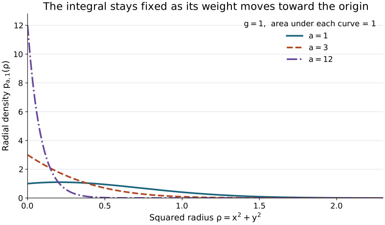
The exact density in (O01.8), with $g=1$. Its tail beyond $\rho_0$ is $e^{-a\rho_0-g\rho_0^2}$. The plot shows concentration of this particular Berezin-reduced integral; a general fermionic functional integral need not define a positive probability density.

Compute only the Gaussian neighborhood

Now suppose we use symmetry to choose a convenient limit instead of evaluating the full non-Gaussian integral. The ordinary part of $QV$ is $\rho\geq0$, with its only zero at the origin. The equations $Q\psi_1=Q\psi_2=0$ select that same point. This is the localization locus of the chosen deformation.

Rescale all four variables together:

$$x=\frac u{\sqrt a},\quad y=\frac v{\sqrt a}, \qquad \psi_i=\frac{\eta_i}{\sqrt a}.$$

The ordinary measure contributes $a^{-1}$, while the two-variable Berezin measure contributes $a$. Their product is unchanged. The action becomes

$$S_g+tQV =u^2+v^2-2\eta_1\eta_2 +\frac g{a^2} \left[(u^2+v^2)^2-4(u^2+v^2)\eta_1\eta_2\right]. \tag{O01.9}$$

At fixed $g$, the last term vanishes as $t\to\infty$. This limit is controlled, not merely pointwise: after extracting the top coefficient, with $s=u^2+v^2$, its absolute value for $a\geq1$ is bounded by $2(1+2gs)e^{-s}$, an integrable function on the plane.

We are left with two elementary integrals:

$$\lim_{t\to\infty}Z(t,g) =\frac1{2\pi} \underbrace{\int du\,dv\,e^{-u^2-v^2}}_{\pi} \underbrace{\int d\eta_2\,d\eta_1\,e^{2\eta_1\eta_2}}_{2} =1. \tag{O01.10}$$

Since the answer is independent of $t$, this also computes the original integral at $t=0$, including any fixed $g\geq0$.

The Gaussian fluctuation calculation is often called the one-loop contribution. Here it is an ordinary finite Gaussian calculation, not a spacetime loop diagram. At finite $a$, the bosonic quadratic integral is $\pi/a$ and its fermionic partner is $2a$; neither factor alone is constant. Their product and the symmetry identity explain the exact answer. The analogous fluctuation rescaling and Gaussian factor in a field theory appear in Willett, version 3, (3.6)–(3.10).

What the argument protects

An insertion must also be Q-closed. For a parameter-independent even $\mathcal O$ with $Q\mathcal O=0$ and adequate decay of the resulting boundary term,

$$\frac{\partial}{\partial t} \int \mathcal O\,e^{-S_g-tQV} =-\int Q\!\left(\mathcal O V e^{-S_g-tQV}\right)=0.$$

The same is true of its normalized expectation value because $Z=1$. It is false for arbitrary insertions. For example, at $g=0$,

$$\langle\rho\rangle =\int_0^\infty d\rho\,a\rho e^{-a\rho} =\frac1a,$$

and $Q\rho\ne0$. Localization did not make the entire distribution or every correlation function independent of $t$.

Nor may we discard the boundary assumption. Restricting the same integral to $x^2+y^2\leq R^2$ gives

$$Z_R(t,g)=1-e^{-aR^2-gR^4}. \tag{O01.11}$$

The cutoff disk is invariant under the bosonic rotation $Q^2$, yet $\partial_tZ_R=R^2e^{-aR^2-gR^4}\ne0$. Rotation invariance of the domain is insufficient to remove the odd Ward identity’s boundary flux.

Practice

1. Complete an observable supersymmetrically

Let $h(\rho)$ be a polynomial. Find $b(\rho)$ such that $\mathcal O_h=h(\rho)+b(\rho)\psi_1\psi_2$ is Q-closed, and calculate its expectation value for the full-plane integral. Apply the result to $h(\rho)=\rho$.

Hint 1

Both $Q\rho$ and $Q(\psi_1\psi_2)$ are proportional to $x\psi_1+y\psi_2$. Terms containing three odd generators vanish.

Hint 2

After multiplying by (O01.5), try differentiating $h(\rho)e^{-F(\rho)}$.

Solution

The variation is $Q\mathcal O_h=(2h'+b)(x\psi_1+y\psi_2)$, so $b=-2h'$. Integrating the top coefficient gives

$$\langle\mathcal O_h\rangle =\int_0^\infty \bigl[F'(\rho)h(\rho)-h'(\rho)\bigr]e^{-F(\rho)}\,d\rho =-\bigl[h(\rho)e^{-F(\rho)}\bigr]_0^\infty =h(0).$$

Polynomial growth is suppressed by the exponential at infinity. The answer is the insertion at the localization point, and is independent of $a$ and $g$.

For $h=\rho$, the completed insertion is $\rho-2\psi_1\psi_2=QV$, with expectation zero. By contrast $\langle\rho\rangle=1/a$ at $g=0$. Direct coefficient extraction gives $\langle\psi_1\psi_2\rangle=1/(2a)$ there, so the two contributions cancel. Dropping the odd part changes the observable and removes its protection.

2. Remove the localization point

Integrate over the annulus $\epsilon^2\leq\rho\leq R^2$, with $0<\epsilon<R$. Find $Z_{\epsilon,R}$. Then let $R\to\infty$ and compare the two orders of limits $\epsilon\to0$ and $t\to\infty$, keeping $g\geq0$ fixed.

Hint 1

The radial integrand is still the derivative in (O01.8). There are now two finite boundary circles.

Hint 2

For any fixed positive $\epsilon$, large $a$ suppresses the entire permitted region. This is not uniform as the inner circle shrinks.

Solution

The exact result is

$$Z_{\epsilon,R} =e^{-a\epsilon^2-g\epsilon^4} -e^{-aR^2-gR^4}.$$

Its derivative with respect to $t$ is $-\epsilon^2e^{-a\epsilon^2-g\epsilon^4} +R^2e^{-aR^2-gR^4}$. These are the two boundary contributions, with opposite orientations. After sending $R$ to infinity,

$$\lim_{t\to\infty}\lim_{\epsilon\to0}Z_{\epsilon,\infty}=1, \qquad \lim_{\epsilon\to0}\lim_{t\to\infty}Z_{\epsilon,\infty}=0.$$

In the second order the neighborhood that would supply the answer was excluded before localization. For each finite $t$, merely deleting the single origin would not change an ordinary integral; deleting a neighborhood and taking a nonuniform limit is different. The smooth full-plane calculation has no inner boundary and gives the first answer.

3. Keep only the positive bosonic deformation

At $g=0$, replace $tQV$ by $t\rho$ while keeping $S_0$ unchanged. This still makes the ordinary exponential narrower. Does it preserve the integral or the odd symmetry? Calculate the answer and identify the missing term.

Hint 1

The coefficient of $\psi_1\psi_2$ in the exponent no longer changes with $t$.

Hint 2

Evaluate $Q(S_0+t\rho)$ before invoking an integrated Ward identity.

Solution

The modified integrand is $e^{-(1+t)\rho}(1+2\psi_1\psi_2)$, giving

$$Z_{\rm bos}(t) =\frac1{2\pi}\frac{\pi}{1+t}\,2 =\frac1{1+t}.$$

Meanwhile $Q(S_0+t\rho)=2t(x\psi_1+y\psi_2)$, which is nonzero for $t\ne0$. The missing action term is $-2t\psi_1\psi_2$. Adding it supplies the fermionic factor $2(1+t)$ that compensates the shrinking bosonic Gaussian. A positive deformation with a convenient saddle is not enough; it must preserve the symmetry used to prove deformation independence.

You can now track a localization calculation from its odd algebra through the boundary identity to the Gaussian factor. In a field theory, each step returns: the square of the chosen supercharge, the measure and contour, the complete set of contributing configurations, and the fluctuation determinants. The finite model explains the method without supplying those theory-specific answers in advance.

Continue with Localization in a field theory to state those requirements for a regulated path integral and test them in a complete free-field example.